April 19, 2003
Aggregate Supply and Aggregate Demand
We allow the price level to change for the IS/LM Model, producing the aggregage demand curve. Adding an aggregate supply schedule allows us to study the relation between output and the price level.
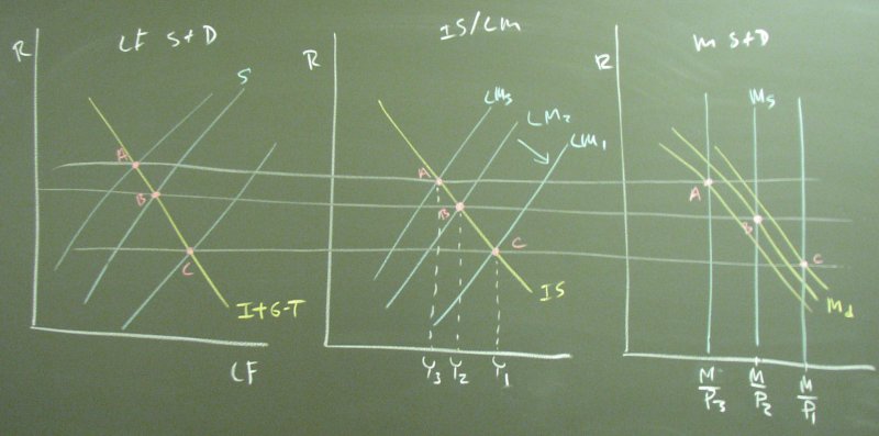
We evaluate output for three price levels. The price level enters the IS/LM Model via the real money supply. Increasing the price level has the same effect as decreasing the nominal money supply.
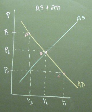
Graphing these three prices vs. output produces the aggregate demand curve. We add an upward sloping aggregate supply curve to reflect the notion that an increased price level would be necessary to get producers to increase output. Keep in mind that a horizontal aggregate supply curve may have been more appropriate during the Great Depression when unemployment reached 25% and large segments of the capital stock were not being used in production.
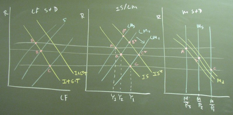
Suppose that a change in government spending (or an autonomous increase in investment or a tax cut) shifts I+G-T to I+G*-T, which is a shift to the right. (Monetary policy would have a similar impact, but the money supply and demand diagram is already complicated. The Keynesians also focused on fiscal policy.)
The aggregate demand curve shifts to the right.
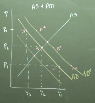
The Keynesians thus expect fluctuations in investment and government fiscal policy (and monetary policy) to shift the aggregate demand curve while the aggregate supply curve remains fixed. This produces a positive correlation between the price level and the level of output.
The classical economists, on the other hand, thought that the aggregate demand curve remained fixed and the aggregate supply curve shifts during business cycles. They focused on an equilibrium determined in the labor market, which is linked to the production side of the economy. (Think of shocks to an agricultural economy.)
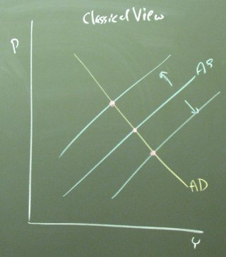
The classical economists thus expected there to be a negative correlation between the price level and the level of output. In a good year, output is abundant, driving down the price.
The Phillips curve handout shows much more accurately the data sketched here. We are making a loose translation from the price level to the rate of inflation.
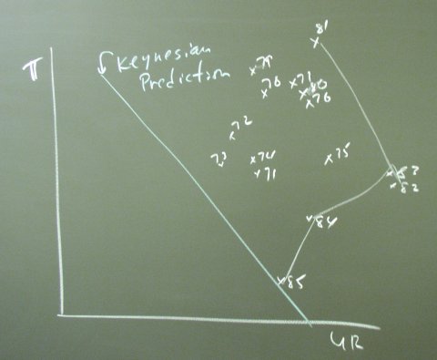
The bottom line is that the Keynesian prediction was supported fairly well by the data between 1948 and 1969. The 70's and the 80's were not kind to the Phillips curve.
One view of this complex topic is that the pre-1969 mainstream economic thought envisioned a political argument about where we wanted to be on the Phillips curve, which functioned something like a budget constraint. The outcome of effects to "fine tune" the economy were a disaster, and once we finally returned to the original Phillips curve area the taste for Keynesian policy studies had diminished.